Every oscilloscope listing on Amazon leads with one number: bandwidth. 100 MHz. 120 MHz. 200 MHz. It is the number sellers shout about because it is the number buyers compare, and for the kind of work that happens on an Arduino bench it is very close to the least important spec on the sheet.
Here is the uncomfortable arithmetic. An Arduino Uno’s analogWrite() pins put out a PWM carrier at roughly 490 Hz on most pins and about 980 Hz on pins 5 and 6. A hobby servo wants a 50 Hz frame. I2C runs at 100 kHz in standard mode and 400 kHz in fast mode. SPI on an Uno tops out in the low single-digit megahertz. Serial debugging at 115200 baud is a signal measured in kilohertz. Nothing in that list comes within two orders of magnitude of 100 MHz.
So if bandwidth isn’t the constraint, what is? Two things almost nobody puts in a product title: sample rate and memory depth. Get those wrong and you will own a scope that technically “sees” 100 MHz and still can’t show you the thing you bought it to find.
The three numbers, and what they actually do
Bandwidth: the frequency where the scope starts lying to you
Bandwidth is the point at which a sine wave fed into the input shows up on screen about 30% smaller than it really is — the −3 dB point. It is not a cliff. A 100 MHz scope doesn’t go blind at 100.1 MHz; it has been quietly rounding off your signal well before that. The practical rule is that you want bandwidth at roughly five times the fastest frequency you care about measuring accurately, which for Arduino work means almost any scope on the market clears the bar by a wide margin.
Sample rate: how many dots the scope has to draw your wave with
A digital scope doesn’t see a continuous wave. It takes snapshots — samples — and connects them. Sample rate is how many of those it takes per second, written as MSa/s (megasamples) or GSa/s (gigasamples). Nyquist says you need more than two samples per cycle to reconstruct a signal at all, but two is a theoretical floor that produces garbage in practice. Scope makers generally want four to five samples per cycle at the rated bandwidth before the interpolation math produces a waveform you can trust, and more like ten if you want to see the shape of a fast edge rather than just that an edge happened.
Memory depth: the one that will actually bite you
This is the spec that gets left off the box, and it is the one that decides whether your scope is useful for embedded work. Memory depth is how many sample points the scope can store in a single capture. It matters because sample rate and time window trade directly against each other: total capture time equals memory depth divided by sample rate, and nothing in the menus can cheat that.
Work an example. A scope with 10,000 points of memory running at its full 1 GSa/s can hold exactly 10 microseconds of signal. Ten microseconds. If you want to watch a complete 20 ms servo frame, the scope has to spread those same 10,000 points across 20 ms, which drops the effective sample rate to 500 kSa/s — one sample every 2 microseconds. You’ll see the pulse width fine. You will not see the glitch riding on its rising edge, because the scope only looked twice while that edge happened.
Now give the same scope 25 million points. At 1.25 GSa/s that is 20 ms of capture at the full sample rate. Same screen, same timebase, 2,500 times more detail inside the window. That is the entire argument for spending more money, and it has nothing to do with bandwidth.
Why “120 MHz” on a $130 handheld isn’t 120 MHz
Once you know the sample-rate rule you can audit a spec sheet in about five seconds, and some of the cheap handhelds do not survive it. Take the popular DSO2512G class of pocket scope: the listing advertises 120 MHz of analog bandwidth and a 500 MSa/s sample rate. Divide them. That’s 4.17 samples per cycle at the rated bandwidth — right at the ragged edge of the four-to-five-samples rule, with nothing left over. The number isn’t fabricated, exactly. It’s just the most generous possible reading of what the hardware can do, and you should mentally discount it to something like 20–30 MHz of trustworthy measurement.
Compare that to the truly cheap pocket scopes, which are weirdly more honest. A 200 kHz bandwidth paired with a 2.5 MSa/s sample rate works out to 12.5 samples per cycle. That is a self-consistent spec. The device is slow, and it tells you so.
What I’d actually buy, at four price points
One scope here is a toy that happens to be useful, one is a compromise with a real purpose, one is the default answer for most people reading this, and one is worth the money only if you’ve already outgrown the others.
This post contains affiliate links. If you buy through them, this site earns a commission at no extra cost to you.
Pocket tier: when you mostly need a signal to exist
The FNIRSI DSO152 is a single-channel, 200 kHz, 2.5 MSa/s handheld with a 2.8-inch screen and a USB-C battery. By bench-instrument standards it is barely a scope. For a specific and surprisingly common job, though, it’s the right tool: confirming that a signal is there, roughly the right shape, and roughly the right frequency. Servo pulses, 490 Hz PWM, a 50 Hz hum you’re chasing, the output of an audio amplifier — all comfortably inside 200 kHz. It will not help you with I2C, it will not resolve a fast edge, and one channel means you can never compare two signals in time. Buy it as a glorified logic probe you can also read voltages off, not as your scope.
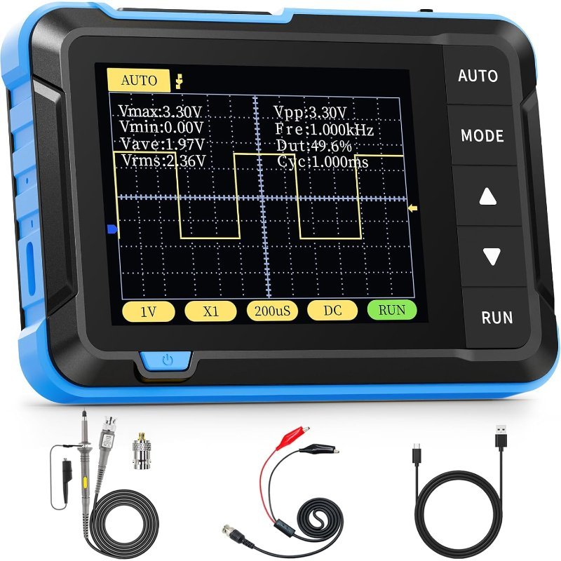
Single channel, 200 kHz, 2.5 MSa/s. Honest about its limits and small enough to forget in a jacket. Good for servo and PWM sanity checks, useless above audio frequencies.
Check Price on Amazon →Portable tier: two channels you can throw in a bag
The DSO2512G earns its place for one reason: it has two channels and a built-in signal generator in something the size of a paperback. Two channels is the jump that changes what you can diagnose, because most embedded debugging is a timing question — did the clock edge land where the data was stable, did the enable line go high before or after the pulse. You cannot answer that with one probe. Discount the 120 MHz claim as discussed above, treat it as a 20-ish MHz instrument, and it covers I2C and most SPI work fine. The 2.8-inch screen is the real compromise; you will squint.
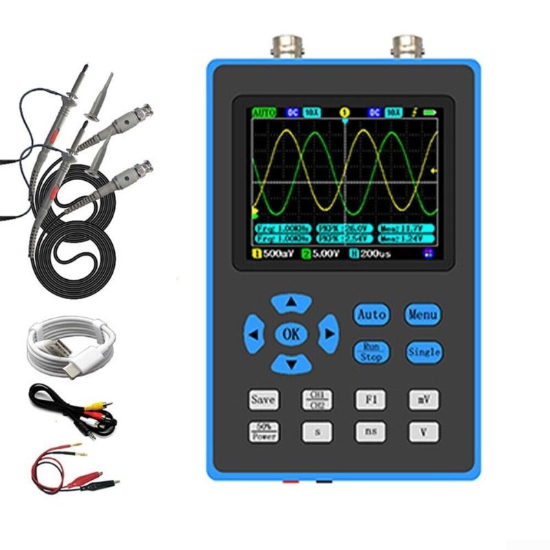
Two channels plus a signal generator in a pocket form factor. Take the 120 MHz rating with salt — 500 MSa/s puts honest measurement nearer 20–30 MHz — but two channels is the upgrade that matters.
Check Price on Amazon →Sweet spot: the one most people should buy
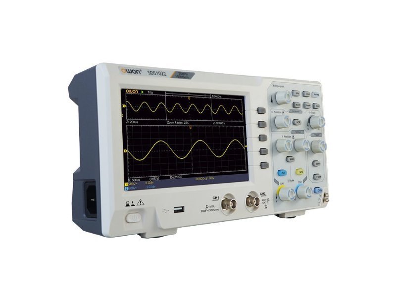
The OWON SDS1102 is a two-channel, 100 MHz benchtop scope with a 1 GSa/s sample rate, an 8-bit vertical resolution, and a 7-inch display. That sample-rate-to-bandwidth ratio is ten to one, which means the 100 MHz figure is real rather than aspirational. It sits on a bench, the screen is big enough to read from a normal sitting distance, the knobs are knobs, and it supports SCPI and LabVIEW if you ever want to script it.
Its weak point is exactly the spec from earlier: OWON lists a 10K record length for this model. That’s the 10-microseconds-at-full-rate scope from the worked example. For Arduino work this is mostly survivable — a 400 kHz I2C byte-and-ack sequence is tens of microseconds, so you can hold a transaction on screen with usable resolution left over. What you cannot do is capture a long event and then zoom into one edge of it. You frame the shot before you take it, the way you would on film.
100 MHz, two channels, 1 GSa/s, 7-inch screen. A ten-to-one sample-rate ratio means the bandwidth number is honest. The 10K record length is the compromise you pay for the price.
Check Price on Amazon →analogWrite(9, 128) and you’ll see a square wave at about 490 Hz, half on and half off. Now build the simplest low-pass filter there is between that pin and your probe — a 10 kΩ resistor in series, and a 1 µF capacitor from the probe point to ground. That puts the cutoff at 1/(2πRC), about 16 Hz, far below the 490 Hz carrier. The square wave collapses into a flat DC level sitting at half your supply, and sweeping the analogWrite() value slides that level up and down. You are watching the trick from Understanding PWM happen in real time, which is a very different thing from reading about it.
Splurge: when memory depth is the thing you are buying
The Rigol DHO804 is four channels at 70 MHz, and on paper that bandwidth is lower than the OWON’s. Ignore that. What you’re paying for is 12-bit vertical resolution instead of 8-bit — 4,096 quantization levels rather than 256, so small signals riding on big ones stop disappearing into the noise floor — and 25 Mpts of memory instead of 10K. Plus a 7-inch 1024×600 touchscreen and four channels, which is the difference between probing a bus and probing a system.
Rigol’s own DHO800 product page does not advertise serial-bus decoding, so don’t buy it expecting the scope to translate I2C traffic into hex for you. If automatic protocol decode is what you want, look at Siglent’s SDS1104X-E, which is four channels at 100 MHz with 14 Mpts and includes free I2C, SPI, UART, CAN and LIN decoding as standard — it’s the obvious rival at this price, and currently easier to find through Siglent’s own dealers than on Amazon. For pure signal fidelity on a hobby bench, the 12-bit front end on the Rigol is the more interesting trade.
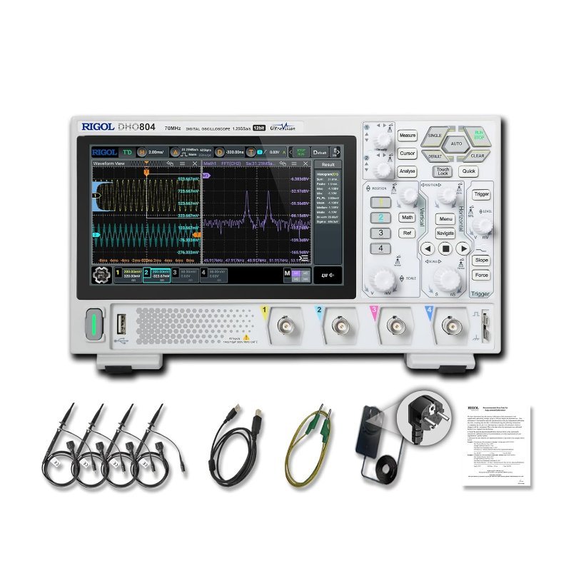
Four channels, 12-bit vertical resolution, 1.25 GSa/s and 25 Mpts of memory. The deep memory and the extra bits are the upgrade; the 70 MHz bandwidth is irrelevant for this work.
Check Price on Amazon →Two things to do the day it arrives
First, understand your probe. Every scope probe ships with a switch marked 1X and 10X. In 10X the probe divides your signal by ten before the scope sees it, which raises the usable bandwidth and reduces how much the probe loads your circuit. Leave it on 10X for almost everything and make sure the scope’s channel menu is set to a 10X probe ratio to match — if the switch and the menu disagree, every voltage you read will be off by a factor of ten. This is the single most common way a new scope user misreads their own circuit, and it’s worth knowing before you conclude your 5 V rail is at 500 mV. Related: if you’re working across boards at different voltages, 5V vs. 3.3V logic levels is the other place that arithmetic goes wrong.
Second, compensate the probe. There is a small square-wave output on the front of every benchtop scope, usually labelled around 1 kHz. Clip the probe to it and look at the corners of the square wave. If they overshoot into little spikes or sag into rounded ramps, turn the trimmer screw on the probe body until they’re square. That’s a thirty-second job that makes every measurement afterwards honest, and most people never do it.
One more thing: a scope is not always the right instrument
If the actual question is “what bytes are going across this bus,” a scope is a clumsy way to ask it. You’ll be counting edges on a screen and converting binary in your head. A cheap USB logic analyzer with software decoding answers that question directly and costs a fraction of any scope here — see the best USB logic analyzers under $50. A scope answers a different question: what does this signal actually look like. Voltage, shape, timing, noise, the ugly edge nobody designed for. Those are the problems a logic analyzer flattens into a clean 1 or 0 and hides from you.
For most people reading this, the honest sequence is a $20 logic analyzer first, the OWON second, and the 12-bit Rigol only once you’ve hit a wall you can name. If you can’t name the wall yet, you haven’t hit it.